Building a Traffic Heatmap with Google Analytics and R

For all of the reporting power that Google Analytics provides, occasionally I want to see data in a way it doesn’t natively support. Most recently, I was interested in understanding hourly and daily shifts in traffic across sections of a site. Knowing when these occur could help authors time their publishing schedules for maximum exposure.

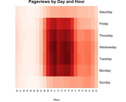
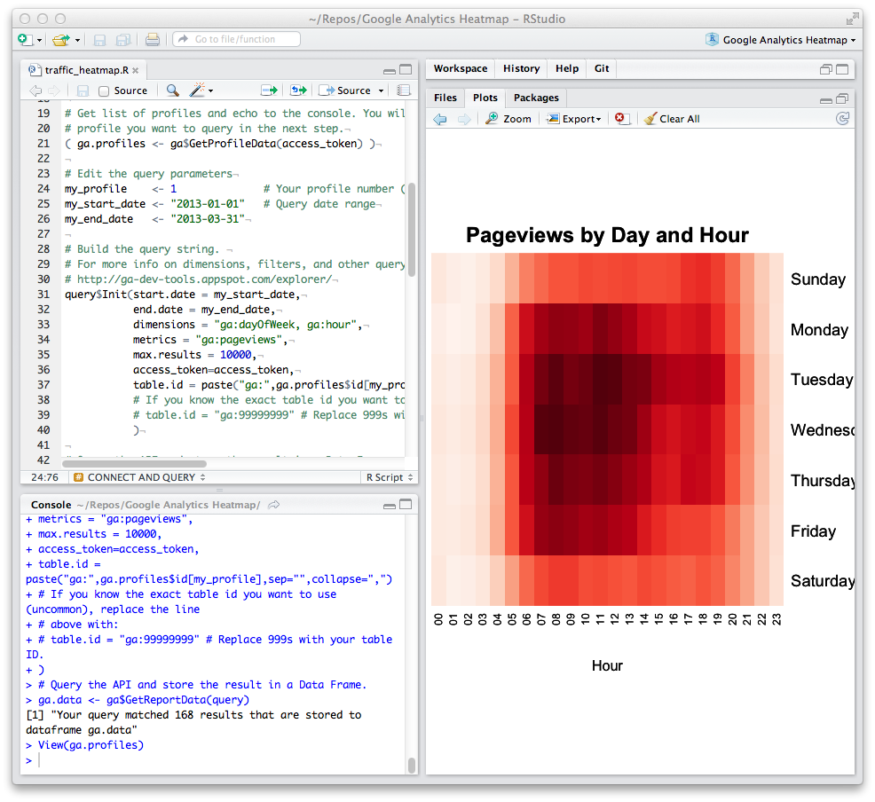
Here’s what I was looking for – a heatmap that boils a few month's worth of data into a weekly view. As you can tell from this example, traffic tracks closely to normal working hours.

My first thought was to pull the data in CSV form from GA, hack it up in Google Spreadsheets or Refine, and then chart it out. But I soon found that I couldn’t find a way to reproduce this chart using their stock widgets. I looked at D3 and a few other charting frameworks and, though I was impressed, I wasn’t ready to commit to that learning curve. Plus, I didn’t want to spend a lot of time pulling data exports from GA if I could help it.

Looking further afield, I remembered R.

Building it in R

R is a scripting / programming environment geared to scientists, statisticians, and data wonks. I had spent some time working through CodeSchool’s R Course a few weeks back, just to see what it did. At the time, I didn’t have a use for it but I figured it would come in handy later.

Sure enough, when I looked into it further, I found a heatmap function that would do precisely what I needed. And finding a post about connecting to GA data programmatically convinced me to spend a Sunday morning bulldozing through just enough R to munge data into the format I needed.

The result is a visually interesting, visceral illustration of how users are hitting the site. Here’s how you can get the same thing, while hopefully not burning part of your weekend along the way. Fair warning though - this tutorial is on the technical side and uses libraries that are still in development. Caveat all the emptors!

Assembling your materials

Here's what you'll need to get started. This assumes you're running on Mac OS X.

• Download and install R - this is the core binary for the language. Their site is a frameset nightmare, so I linked directly to UC Berkeley's mirror.
• Download and install RStudio Desktop - this is an IDE that runs atop R. It's free and makes working with R much easier.
• Get a copy of the heatmap script - once unzipped, this should give you the source code needed to create a heatmap. 
• Download RGoogleAnalytics 1.2 - this is the library that helps us connect to Google. Get the tar.gz version; we'll use this later. Edit: Version 1.3 was posted a few hours ago and after a cursory look, it seems to work too.

Once you have all these, launch RStudio and take a deep breath. It's about to get real.

Installing the libraries

We use two major libraries in this script: RColorBrewer for producing sane color schemes and RGoogleAnalytics for getting the data. The latter relies on RCurl for network requests and RJson for parsing the data returned.

Installing RColorBrewer, RCurl, and RJson

Most libraries in R are super-easy to install. Just issue a command and R installs the right thing from the Comprehensive R Archive Network (CRAN). Let's do it now.

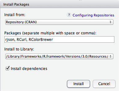
Navigate to the Packages panel and click Install Packages. In the dialog that follows, type rjson, RCurl, RColorBrewer  into the Packages field. Confirm the other settings match the screenshot below and click Install.

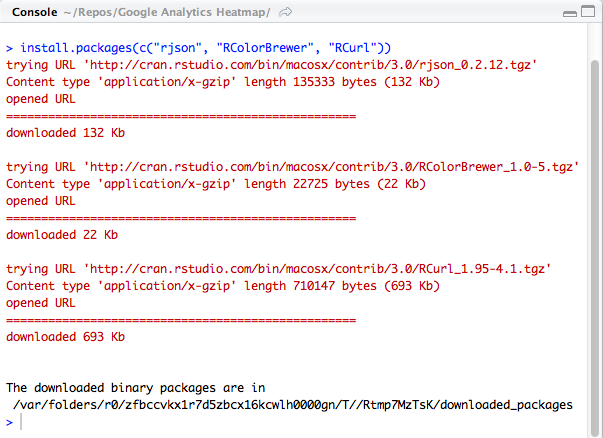
The installation process will write its status to the RStudio console. Once it stops, you should see a line that states that the downloaded binary packages are located in some byzantine path on your machine. Don't be afraid: this is good and signifies that they were installed properly.

Installing RGoogleAnalytics

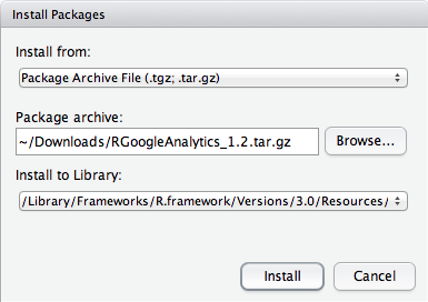
Sadly, it's not the same process for RGoogleAnalytics. That library is still under significant development and, as a result, we'll need to install it from the file you downloaded earlier.

With RStudio open, open the Packages pane and click Install Packages. Choose Install from package archive and select the library you downloaded earlier. Once you're ready, click Install.

Once it's done, the console message should look similar to the previous step. For me, however, it complains that the package isn't available for R 3.0 but then soldiers forward and installs properly. I haven't traced down the cause but, if you know it, let's discuss it in the Issues.

Running the script

Connecting to GA

Provided you made it through the above steps mostly unscathed, we're now at the fun part. We're going to open the project, step through the code, authenticate to Google, and make a diagram. 

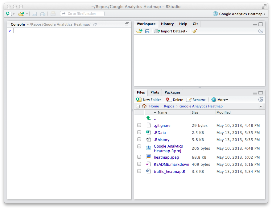
Open the Google Analytics Heatmap.Rproj project in RStudio using the project menu, then open traffic_heatmap.R from the Files pane. We'll do most of our work here. 

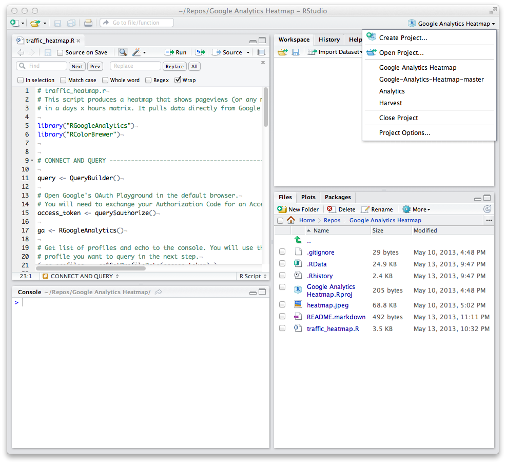
RStudio can execute code all at once or line-by-line. Because part of our script asks for user input, we want to move line-by-line. To do this, first ensure your cursor is on line 1 in traffic_heatmap.R. Then hit “⌘-Return” to step through each line in succession. Alternatively, you can click the Run -> button.

Do this until you execute the following line.

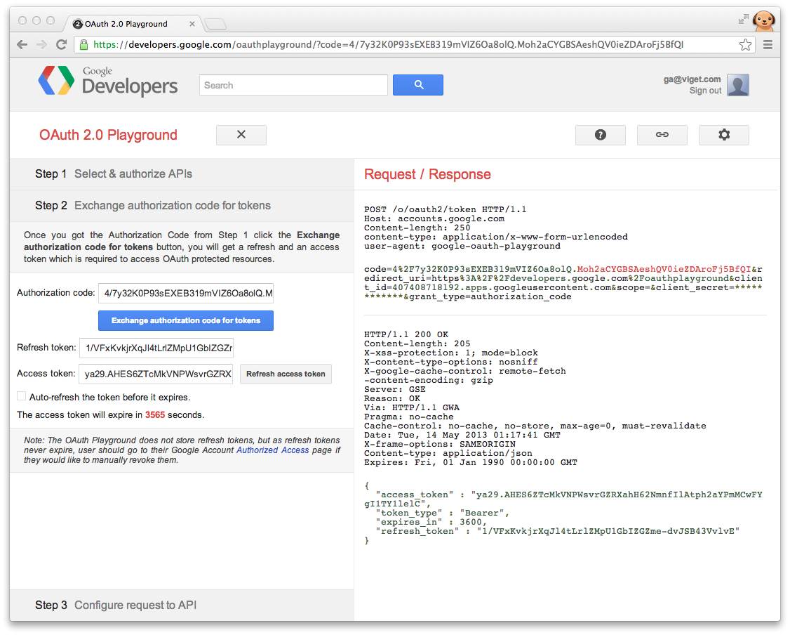
Once this line is run, Google’s OAuth Playground will appear in your default browser, asking you to authorize access. It uses the current active account so, if this is different from your GA account, you may need to log into that first and rerun the last line.

Once done, GA will allow us to exchange the authorization code for an access token. Do this, then paste the resulting token at the prompt within the RStudio console.

Choosing your profile

Since each GA account can manage many different profiles, you will need to choose the one you care about. Stepping through the code with ⌘-Return, you'll encounter this line.

Running this will echo the profiles that you manage in GA. Find the number of the profile you want to use. This will be the number in the far left column.

Querying and displaying

Now we can get some data. First, replace the "1" after  my_profile with the profile number you just chose. You'll probably also want to change the date range.

Once you're satisfied with that, move your cursor back to the my_profile <- your_profile_number line. Step through it and the rest of the code. You'll know you're on the right track when you see the following written to the console: 

The code thereafter cleans up the data and modifies its format to something the heatmap chart can use. You can step through it as fast as your fingers will allow – there's nothing else to change. 

Once you're done, you should see the chart appear in the Plot panel. From there you can export the file to a format you prefer. 

Whew, that's it. You're done.

In Conclusion

While the initial investment of time was high – Sundays are in short supply! – it's trivial to run this again. Because of this, it becomes incredibly easy to:

• compare different sections of a site
• map unique visitors instead of pageviews
• look for time drifts in device usage
• gauge uptake from social media efforts

Essentially any dimension, metric, or filter available through the GA Reporting API can be used. So have fun experimenting with it. 

If you run into technical problems, I'll do my best to help out but I'm still learning too. Feel free to add any issues you encounter here. Same goes for any enhancement ideas. And if you're a benevolent R wizard who wants to improve my code, fork it and send me a pull request. I'd be much obliged. 

Oh, and by the way, we're hiring!

We're looking to grow our UX team in all three of our office locations. Check out our UX Designer job listing and, if you think you're a fit, please get in touch!